
Digital Filter
Digital filter can be used to process time series data. Some contents comes from the introduction.
In signal processing, the function of a filter is to remove unwanted parts of the signal, such as random noise, or to extract useful parts of the signal, such as the components lying within a certain frequency range. Here aslo said that Digital filters are used for two general purposes: (1) separation of signals that have been combined, and (2) restoration of signals that have been distorted in some way.
Input
\[\mathbf{x_0, x_1, x_2, x_3, …, x_n}\]Output
\[\mathbf{y_0, y_1, y_2, y_3, …, y_n}\]Examples of simple digital filters
-
Unity gain filter: \(\mathbf{y_n}=\mathbf{x_n}\)
-
Simple gain filter: \(\mathbf{y_n}= \mathbf{Kx_n}\)
-
Pure delay filter: \(\mathbf{y_n}=\mathbf{x_{n-1}}\)
-
Two-term difference filter: \(\mathbf{y_n}=\mathbf{x_n}-\mathbf{x_{n-1}}\)
-
Two-term average filter (This is a simple type of low pass filter as it tends to smooth out high-frequency variations in a signal): \(\mathbf{y_n}=\frac{\mathbf{x_n+x_{n-1}}}{2}\)
Order of a digital filter
The order of a digital filter is the number of previous inputs (stored in the processor’s memory) used to calculate the current output.
Digital filter coefficients
All of the digital filter examples given above can be written in the following general forms:
- Zero order: \(\mathbf{y_n=a_0x_n}\)
- First order: \(\mathbf{y_n=a_0x_n+a_1x_{n-1}}\)
- Second order: \(\mathbf{y_n=a_0x_n+a_1x_{n-1}+a_2x_{n-2}}\)
The constants \(\mathbf{a_0, a_1, a_2, ...}\) appearing in these expressions are called the filter coefficients. It is the values of these coefficients that determine the characteristics of a particular filter
Recursive and non-recursive filters
A recursive filter is one which in addition to input values also uses previous output values. These, like the previous input values, are stored in the processor’s memory.
Note: Some people prefer an alternative terminology in which a non-recursive filter is known as an FIR (or Finite Impulse Response) filter, and a recursive filter as an IIR (or Infinite Impulse Response) filter.
Order of a recursive (IIR) digital filter
The order of a recursive filter is the largest number of previous input or output values required to compute the current output.
Coefficients of recursive (IIR) digital filters
A first-order recursive filter can be written in the general form
\[\mathbf{y_n=\frac{(a_0x_n+a_1x_{n-1}-b_1y_{n-1})}{b_0}}\]The reason for expressing the filter in this way is that it allows us to rewrite the expression in the following symmetrical form:
\[\mathbf{b_0y_n+b_1y_{n-1}=a_0x_n+a_1x_{n-1}}\]The transfer function of a digital filter
First of all, we must introduce the delay operator, denoted by the symbol \(\mathbf{z^{-1}}\):
\[\mathbf{z^{-1}x_n=x_{n-1}}\]Hence we have:
\[\mathbf{ \frac{y_n}{x_n} = \frac{a_0+a_1z^{-1}+a_2z^{-2}}{b_0+b_1z^{-1}+b_2z^{-2}}}\]This is the general form of the transfer function for a second-order recursive (IIR) filter.
The transfer function of a second-order second-order (FIR) filter can therefore be expressed in the general form
\[\mathbf{ \frac{y_n}{x_n} = a_0+a_1z^{-1}+a_2z^{-2}}\]How Information is Represented in Signals
Fortunately, there are only two ways that are common for information to be represented in naturally occurring signals. We will call these: information represented in the time domain, and information represented in the frequency domain.
The step response describes how information represented in the time domain is being modified by the system. In contrast, the frequency response shows how information represented in the frequency domain is being changed.
Time Domain Parameters: risetime, overshoot, linear phase
Frequency Domain Parameters: passband, stopband, transition band, cutoff frequency, fast roll-off, passband ripple, stopband attenuation.
High-pass, band-pass and band-reject filters are designed by starting with a low-pass filter, and then converting it into the desired response.
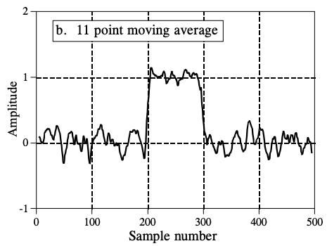
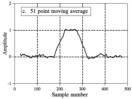
Moving Average Filters
\[y[i]=\frac1M\sum^{M-1}_{j=0}x[i+j]\]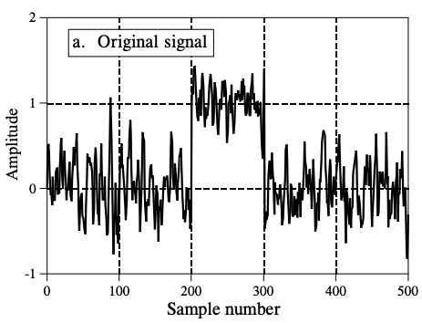
Advantages of Digital Filter
Compared with other methods that can process,